Same task, but third classification algorithm – naive Bayes. I was looking forward, because a MATLAB script was already written and I naively thought my only work is to replace one function name (fitcknn to fitcnb). My good mood lasted until I realized that optimization of hyperparameters did not have any impact – the output from optimization was always the same as without it (only the computational time was longer as usual). In a state of mild panic it is always advisable to read an orange warning message. It said something like “if we want to optimize 'width' parameter, all numeric predictors should be standardized before”. I started to panic even more until I realized that the solution is simple. I just threw the whole dataset into the function zscore, which returns data where each attribute (column) has mean 0 with standard deviation 1.
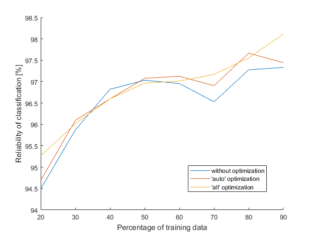
There was one more error to be fixed. This one was insidious, because it occurred only sometimes and then broke whole program. I’m glad that I found it before I run main program, it would be unpleasant to break in the middle of 23 hours of optimization. That’s why the chart starts at 20 % of training data and not at 10 % as previously (if there is only few training data, a zero variance may occur).
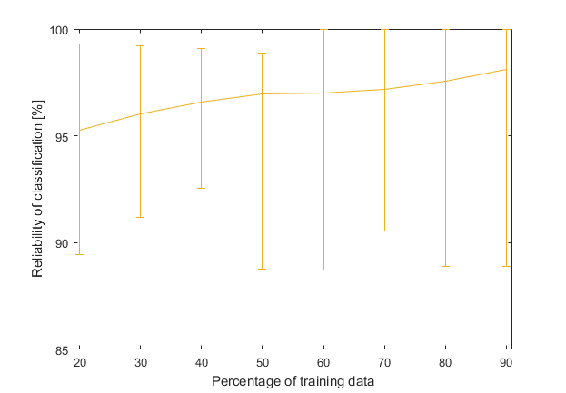
Because the ‘all’ optimization line looks good, here it is once again, but this time with added maximum and minimum values (achieved from 50 different measurements).
The table below compares the reliability of the classification (when percentage of training data is 70 %), as achieved by three different classifiers. The second table compares the time that each classifier requires for its construction.
| Mode | Clasification tree | k-nearest neighbors | Naive Bayes |
| without optimization | 91.2 % | 73.4 % | 96.5 % |
| 'auto' optimization | 89.2 % | 94.9 % | 96.9 % |
| 'all' optimization | 90.9 % | 96.3 % | 97.2 % |
| Mode | Time per one tree | Time per one k-NN | Time per one NB |
| without optimization | 0.01 s | 0.02 s | 0.03 s |
| 'auto' optimization | 46.3 s | 58.6 s | 97.2 s |
| 'all' optimization | 65.5 s | 94.3 s | 108.9 s |
Last but not least and certainly not the easiest question is how naive Bayes works and why is it so good? I would prefer to conclude this with a statement -

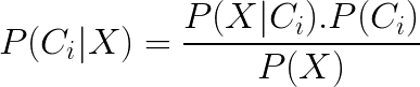
But some people might not be satisfied with this explanation. As you wish, but we can no longer escape from math. Naive Bayes classifier is based on Bayes’ theorem and classifies data according to a probability. The probability of each class is for every sample defined by Bayes’ theorem:
-
$\boldsymbol{P(C_i|X)}$ is a posterior probability, which we want to calculate because a sample is classified into a class with highest $P(C_i|X)$, where $i = 1,2$ or $3$.
-
$\boldsymbol{P(X|C_i)}$ is the probability of $X$ under the condition $C$, in our case (remember my first post, where is explained how our dataset looks) $P(X|C_i)$ is the probability that a sample $X$ belongs to a class $C_i$. The sample $X$ is represented by 13-dimensional vector $X = (x_1, x_2, …, x_{13})$ where each component of the vector is one attribute of wine.
-
$\boldsymbol{P(C_i)}$ is the prior probability of $C$ – the probability that a sample belongs to a class $C_i$ without regard to any parameters of $X$. A class’s prior can be calculated as $P(C_i)$ = (number of samples in the class $i$) / (total number of samples). Our dataset has 178 samples where 59 of them belong to the class 1, 71 to the class 2 and 48 to the class 3. Then the prior probabilities are as follows: 33 %, 40 % and 27 %.
-
$\boldsymbol{P(X)}$ is the prior probability of $X$, it doesn’t depend on a class, therefore it is the same for each class and we only need to maximize the numerator $P(X|C_i).P(C_i)$.
The only probability that we don’t know yet is $P(X|C_i)$. Here we must naively assume that every feature $x_k$ is conditionally independent of any other feature $x_j$, given the class $C$. To make such an assumption that features are unrelated is quite naive, because they usually depend on each other. Then we can express $P(X|C_i)$ as follows:

$P(X|C_i)$ can be calculated from training data. For discrete attributes, $P(X|C_i)$ is a product of all conditional probabilities for each attribute, where $P(x_{k}|C_{i})=s_{ik}/{S_i}$. $S_i$ is the number of samples (from training data), which belong to the class $i$ and $s_{ik}$ is the number of those for which the value of the given attribute is equal to the value of the object we want to classify. But since our data are continuous, we must assume normal Gaussian distribution:
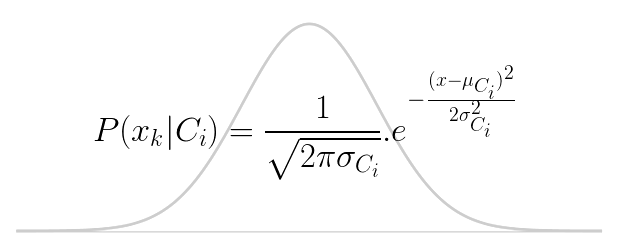
Where $\mu_{Ci}$ is the mean of the values in the attribute $x$ associated with the class $C_i$ and $\sigma_{Ci}$ is the variance of the values in $x$ associated with the class $C_i$.
To classify an unknown sample, an element $P(X|C_i).P(C_i)$ should be calculated for each of three classes and then the sample is assigned into the class with the highest probability. That’s finally all.