In the introductory post, I explained why artificial intelligence and machine learning matters. Leave out sci-fi machines aside, we have to start somewhere – for example with trees. Goals have been set: we want to predict a class of wine based on its properties. We will solve this task using a classification decision tree, which MATLAB will create for us. At the beginning, we must bring data to MATLAB and convert them to a form that is MATLAB-friendly. Obviously, that form is a matrix.
%% load data from a weburl = 'https://archive.ics.uci.edu/ml/machine-learning-databases/wine/wine.data';file_name = 'wine.data';urlwrite(url, file_name); %% conversion of data into a matlab matrixdata = csvread(file_name);We can grow a classification tree using the data set, but if we also want to evaluate outputs, testing samples should be different from samples used to create the tree model. The ratio between training and testing data was set to 7:3. Later we can look at how different ratios affect results. The data were distributed randomly. The first column of the matrix is a class identifier (1-3) and 13 remaining columns are attributes.
%% data division into training and testingpercent_of_training_data = 0.7; number_of_samples = size(data, 1);number_of_training_samples = round(percent_of_training_data*number_of_samples); number_of_testing_samples = number_of_samples - number_of_training_samples;shuffled_indices = randperm(number_of_samples);training_indices = shuffled_indices(1:number_of_training_samples);testing_indices = shuffled_indices(number_of_training_samples+1:end);training_samples = data(training_indices, :);testing_samples = data(testing_indices, :);training_x = training_samples(:, 2:end);training_y = training_samples(:, 1);testing_x = testing_samples(:, 2:end);testing_y = testing_samples(:, 1);The MATLAB function fitctree returns a binary classification tree based on the input variables, which we have stored in the matrix training_x, and output Y stored as the vector training_y. The returned binary tree splits branching nodes based on the attribute values in the matrix training_x.
%% creating a classification tree based on the training dataclassification_tree = fitctree(training_x, training_y)view(classification_tree, 'Mode', 'graph')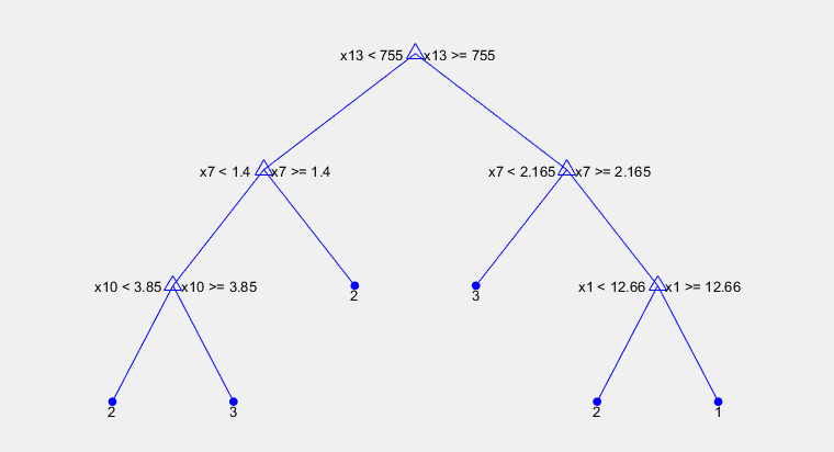
And here it is, our first tree. There is a path from the root to the leaf, where the condition in each node selects the convenient branch and leaves represent an appropriate class. The root node splits samples according to attribute x13, which represents the amount of proline (proteinogenic amino acid). If we want a first class wine, amount of proline has to be higher than 755 μg/g, content of flavonoids above 2.165 mg/g and finally alcohol content must be more than 12.66 %.
Now is the time to find out how good this tree is at predicting outputs. The function predict creates a vector of expected classes using a classification tree and properties of wines. To evaluate a reliability of a classification tree we compare values given by that tree and correct answers stored in vector testing_y.
%% verifying the reliability of the classification tree, based on testing datacategories = predict(classification_tree, testing_x);number_of_errors = nnz(testing_y-categories);accuracy = (number_of_testing_samples-number_of_errors)/number_of_testing_samples*100;fprintf('Number of testing samples: %d\n', number_of_testing_samples);fprintf('Number of samples with wrong classification: %d\n', number_of_errors);fprintf('Percentage of correct classification: %.1f%%\n', accuracy);From 53 testing samples 5 were with wrong classification. We got 90.6 % correctly assigned training samples. Is it good, bad, enough? Can we gain a better outcome? How can we change it? Firstly, each time the program runs, there is a different tree with a different result due to randomly divided data into training and testing. Secondly, there is a ratio between them, which can be modified. Let’s create a loop to iterate over percentage of a training data from 10 to 90 % with 1 % step.
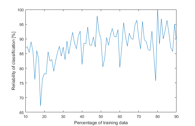
It looks messy because of randomness, so another loop will draw an average of 1000 previous iterations (that’s a lot of trees, almost a forest).
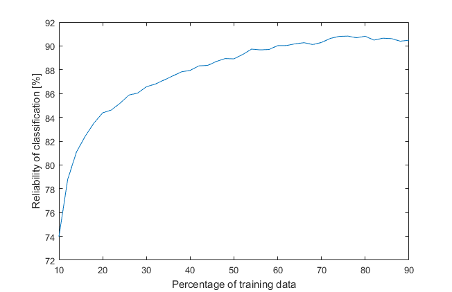
We can see that reliability increases with increasing percentage of a training data and best results we get when percentage is between 70 to 80 % while a model is not yet overfitted. For now it is enough, next time we will force MATLAB to try even harder, because we are not modest and we are asking for a better trees.