In modern medicine and pharmaceutical research, molecular docking plays a key role in the identification of potential drugs. This process allows scientists to simulate interactions between small molecules (ligands) and target proteins, which helps predict how effective these molecules might be as drugs. Traditional docking methods often involve complicated and time-consuming calculations, limiting their efficiency and speed.
Neural networks, which are inspired by the way the human brain works, offer a new and innovative approach to this challenge. These networks consist of layers of interconnected artificial neurons that learn from large amounts of data and identify complex patterns and relationships. The use of neural networks in molecular docking has the potential to improve the accuracy and speed of docking score predictions, which can greatly accelerate the process of new drug development.
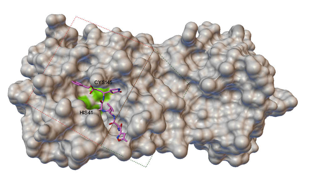
The aim was to replace the laborious “docking” of molecules into the target protein cavity with neural networks, focusing on the 3CLpro SARS-CoV-2 protein (6WQF), which is key in SARS-CoV-2 virus replication. In the figure, you can see the specific molecule of our protein as well as the indicated slice of the protein needed for the next steps. Here we can see the activation site and the substance that has bound to this site.
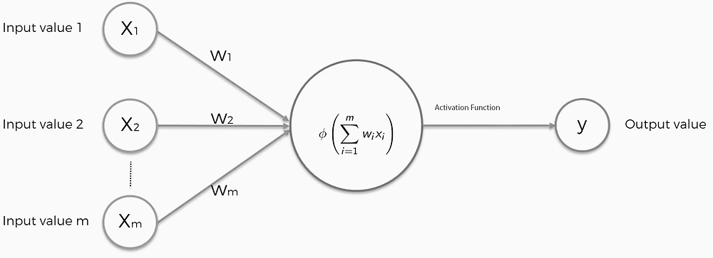
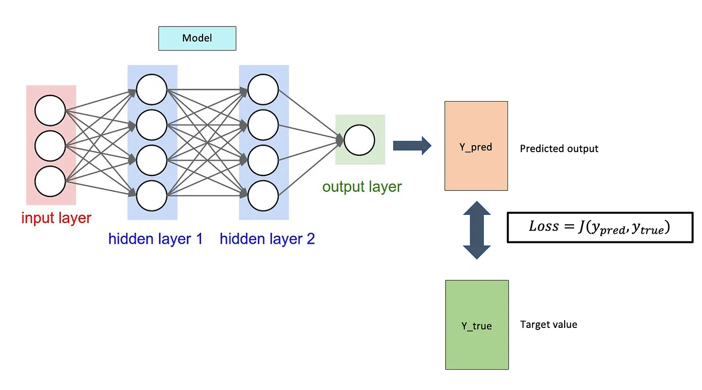
Neural networks are computational models that can solve complex tasks such as image recognition. As you can see in the picture, they are composed of neurons divided into layers: input, hidden, and output. The whole thing is done by optimizing the weights of the individual neurons with algorithms like gradient descent to minimize the errors between the network predictions and the actual values. And so over time, the network learns, improving its accuracy and performance. We then used the TensorFlow library developed by Google. Our dataset contained 60,000 chemical molecules. The models we used and then compared were the necessary descriptors that transform the data into a single feature vector and this then enters the network, eventually, we get the desired chemical properties. In our case, these were the energies.
Also for the proper setup of the neural network, the following things are needed :
· Activation functions which are the basic element of neural networks. They define how the input signal to the neuron is transformed into the output signal from the neuron. The choice of activation function greatly affects the performance.
· Loss functions define how neural networks evaluate prediction error against expected outputs. We used MSE regression, but binary and multi-class classifiers can also be used.
· Optimizers in neural networks are algorithms that serve to minimize the error between network predictions and actual values by updating the network weights during the training process.

· Descriptors are input characteristics or features of the data that are used for training or prediction.
Coulomb Matrix
Coulomb Matrix (CM) is a simple global descriptor that mimics the electrostatic interaction between nuclei. Coulomb matrix is calculated using the equation below.
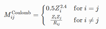
It maintains rotational invariance. The diagonal elements can be thought of as the interaction of the atoms with themselves and are essentially a polynomial fit of the atomic energies to the nuclear charge Zi. Off-diagonal elements represent Coulomb repulsion between nuclei i and j.
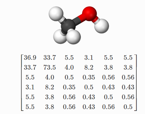
Consider the CM for methanol. In the matrix above the first row, it corresponds to the carbon (C) in methanol interacting with all the other atoms (columns 2-5) and with itself (column 1). Similarly, the first column shows the same numbers because the matrix is symmetric. Further, the second row (column) corresponds to oxygen and the remaining rows (columns) correspond to hydrogen (H).
Smooth Overlap of Atomic Positions
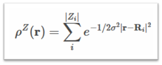
Smooth Overlap of Atomic Positions (SOAP) is a descriptor that encodes regions of atomic geometry using a local expansion of the Gaussian fuzzy atomic density (ρZ(r)) with orthonormal functions based on spherical harmonic (Ylm(ϴ, Ф)) and radial basis functions(gn(r)). The SOAP output from DScribe is a vector of partial power spectra p.
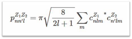
The coefficients are defined as the following inner products:
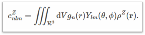
where (ρZ(r)) is the Gaussian smoothed atomic density for atoms with atomic number 𝑍 defined as
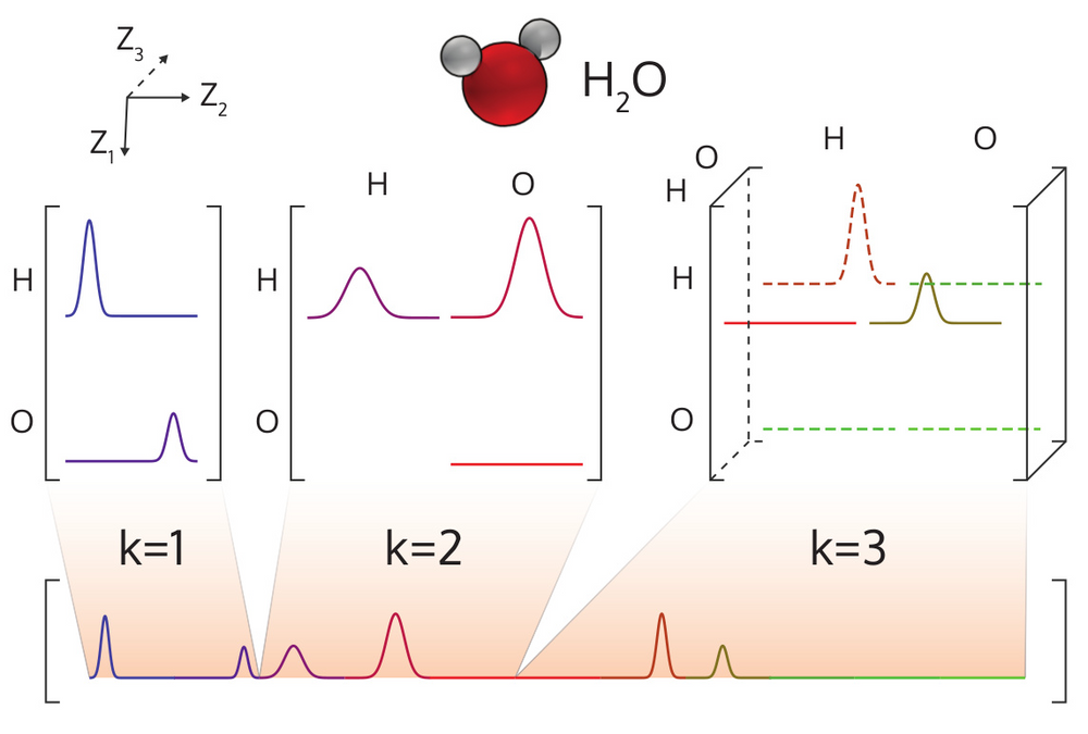
Many-body Tensor Representation
The many-body tensor representation (MBTR) encodes a structure using a distribution of different structural motifs. MBTR is particularly suitable for applications where the interpretability of the input is important since the features are easy to visualize and correspond to specific structural properties of the system. In MBTR the geometry function gk is used to transform a string of atoms k, into a single scalar value. The distribution of these scalar values is then constructed with an estimate of the kernel density to represent the structure.
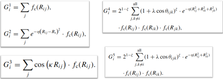
Atom-centered Symmetry Functions
Atom-centered Symmetry Functions (ACSFs) can be used to represent the local environment near an atom by using a fingerprint composed of the output of multiple two- and three-body functions that can be customized to detect specific structural features.
Notice that the DScribe output for ACSF does not include the species of the central atom in any way. Suppose the chemical identity of the central species is important. In that case, you may want to consider a custom output stratification scheme based on the chemical identity of the central species, or the inclusion of the species identified in an additional feature. Training a separate model for each central species is also possible.
We need to maintain rotational and translational invariance. So we chose the parameters G2 and G4. The value of the G2 parameter depends on the distance between two atoms in the molecule. The value of the G4 parameter depends on the angle between three atoms in the molecule.
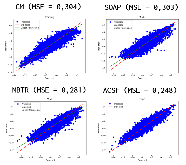
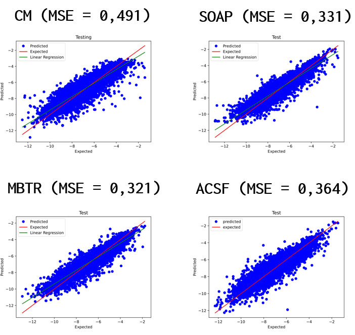
Results
You can see the results for each model as well as the MSE values. Based on these values for our case, the best model is MBTR, since the MSE value for the test data gave the smallest value. For comparison, we first see the result plots for the training data and then for the test data. We had the ratio of training and test data fixed at 0.25 and 0.6, respectively.
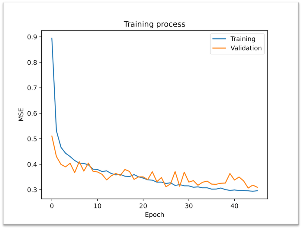
The next Figure represents the Training process of the best model for our testing data (ACSF). MRSE values are decreasing, although oscillation was slight during the validation set, but it’s still okay.