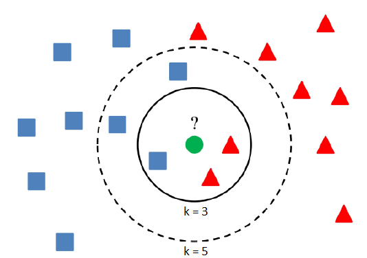
The aim of this project is still the same, only a classification algorithm will be different. No more trees anymore. They will be replaced by nearest neighbors, but the method is the same as previously. K-nearest neighbors (k-NN) is a simple classification algorithm, which assign a class to an item according to a majority class of its nearest neighbors.

The result depends upon the number of neighbors and therefore k is a parameter, which can be optimized. The MATLAB function fitcknn returns a k-nearest neighbor classification model based on the predictors (input variables) and response (output). A default k-nearest neighbor classifier uses a single nearest neighbor only, so the object is simply assigned to the class of that single nearest neighbor. Again, we can use an additional argument 'OptimizeHyperparameters' with value 'auto' (optimize Distance and NumNeighbors) or 'all' (optimize all eligible parameters). To determine the distance between items in space various metrics can be used. The most common and default distance metric is Euclidean, but there are plenty of other distance metrics such as Chebychev, Minkowski or City block distance. You can choose a distance as you wish or let the training algorithm to learn the optimal parameters from the data. Another useful hyperparameter is DistanceWeight. If its value is inverse, then the nearer neighbors contribute more than distant ones.
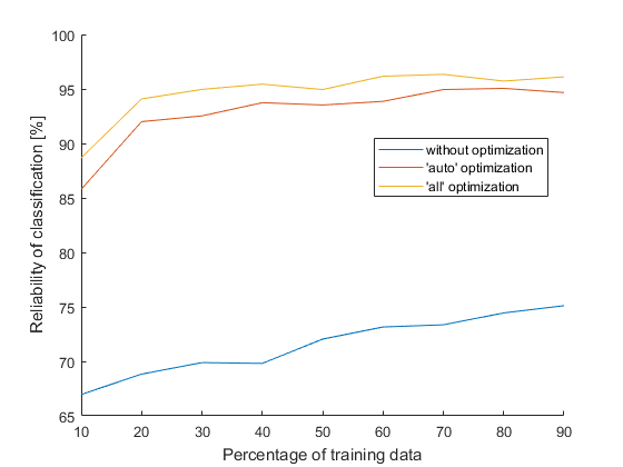
Time can obtain different meanings. Time is a physical quantity, time is money, time is the fourth dimension (or eleventh), time is relative, but what time is not? A substance that I’ve got plenty. Despite of this I had been waiting (im)patiently for nearly 20 hours to get this lovely chart.

No, it’s not necessary to wait that long, I just wanted to compare statistically relevant data. This nice chart shows us how proper optimization should look like (trees can take an example). The table below compares reliability of classification when percentage of training data is 70 % and 80 %, where reliability is again an average from 50 values:
| Mode | Time per one classifier | Reliability at 70 % | Reliability at 80 % |
| without optimization | 0.015 s | 73.4 % | 74.4 % |
| ‘auto’ optimization | 58.56 s | 94.9 % | 95.1 % |
| ‘all’ optimization | 94.34 s | 96.3 % | 95.7 % |
Data are always randomly splitted into training and testing, therefore outputs differ and sometimes we get 100 % reliability. The next table includes how many times out of 50 trials we achieved 100 % reliability of classification and also the worst result.
| Number of 100 % from 50 trials | The worst reliability | |||
| Mode | at 70 % | at 80 % | at 70 % | at 80 % |
| without optimization | 0 | 0 | 58.5 % | 63.9 % |
| ‘auto’ optimization | 3 | 11 | 81.1 % | 86.1 % |
| ‘all’ optimization | 6 | 11 | 92.5 % | 83.3 % |
The last table compares the reliability of classification achieved by classification tree and k-nearest neighbors (when percentage of training data is 70 %).
| Mode | Clasification tree | k-nearest neighbors |
| without optimization | 91.2 % | 73.4 % |
| ‘auto’ optimization | 89.2 % | 94.9 % |
| ‘all’ optimization | 90.9 % | 96.3 % |
This time optimization matters. Classification using k-NN without optimization fails, but with optimization far exceeds the trees. (True for this dataset, I do not dare to generalize).