The aim of this work is to design and implement a predictive model for an alkylation process based on available measurements in order to replace a faulty sensor. This can help minimize the need for laboratory measurements.
Alkylation is one of the most important processes in fuel refining.
It converts small, reactive molecules into clean and stable fuel components. In the reactor, isobutane reacts with an alkene to produce alkylate. Isobutane is the main reactant, which means it is continuously recycled back to the input. Since the reaction is exothermic, continuous cooling is required.
For the purpose of this case study, standardized process data from the alkylation reactor at Slovnaft were provided. These data served as the basis for further preprocessing and model development.
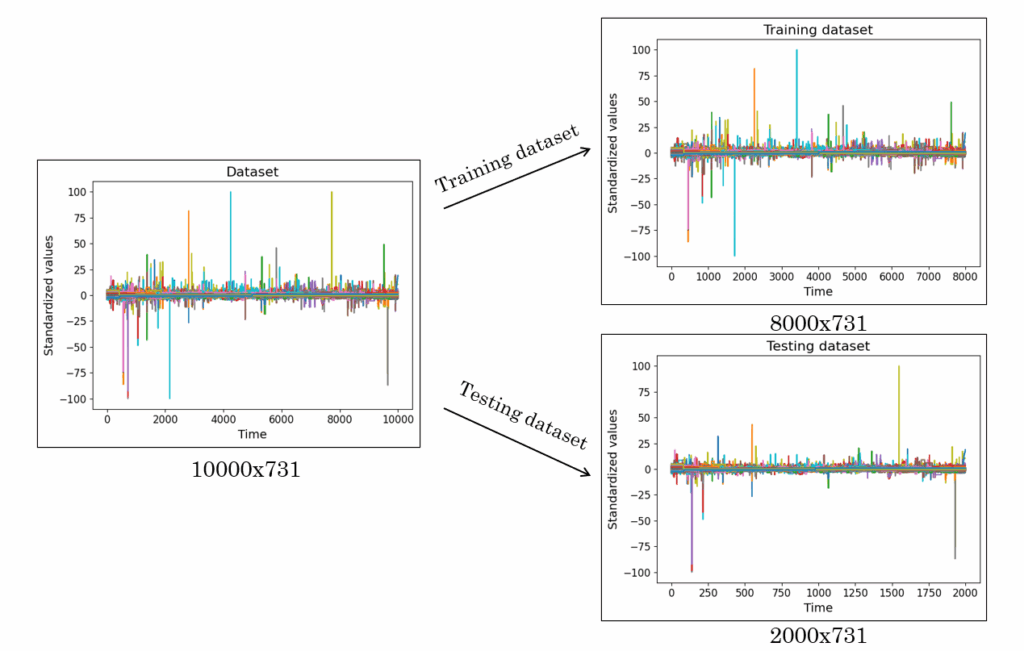
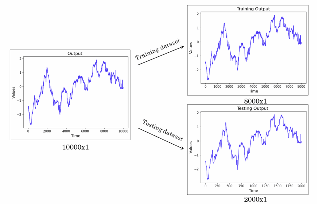
The input variables represent different parts of the alkylation process. The full dataset was split into training and testing subsets using random indexing. The output variable is a sensor whose accuracy is currently in question. Similar to the inputs, the output data were also splited into training and testing subsets using random indexing. In our case, the output represents information about recycled isobutane.
After splitting our data into training and testing subsets, we moved on to data preprocessing, which included eliminating unsuitable sensors and removing outliers.
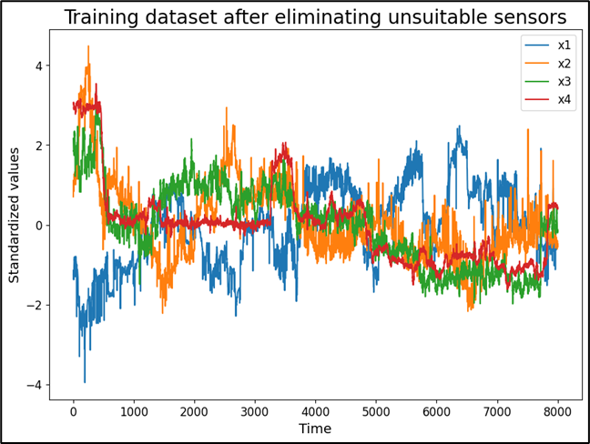
We analyzed all input variables and removed those that were not suitable for further modeling. These included malfunctioning sensors, sensors with overly linear behavior, and sensors with sudden value fluctuations. We also aimed for low correlation between input variables, since we did not want them to be too similar. On the other hand, high correlation between input and output variables was desired, because the inputs should reflect the output as closely as possible. Based on these criteria, we reduced the number of input variables to four relevant ones.
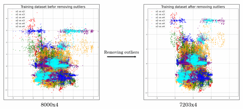
Then, we detected and removed outliers, as they can distort the model’s learning process and lead to inaccurate predictions. As a result, the training dataset was reduced from 8000 to 7203 measurements, and the testing dataset from 2000 to 1797 measurements.
After completing the data preprocessing and feature selection phase, we proceeded to the model development stage.
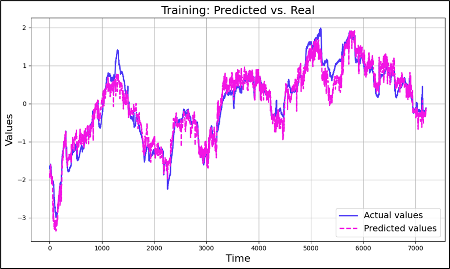
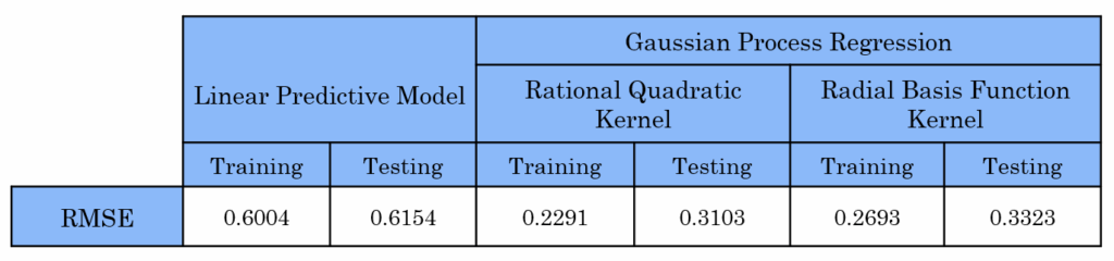
As a first step, we applied a general approach using the entire reduced and cleaned training and testing datasets. We implemented Ordinary Least Squares (OLS) regression. We also applied Gaussian Process Regression (GPR). In GPR, predictions are derived from a covariance matrix constructed using a kernel function. In our case, we used the Rational Quadratic kernel and the Radial Basis Function (RBF) kernel.
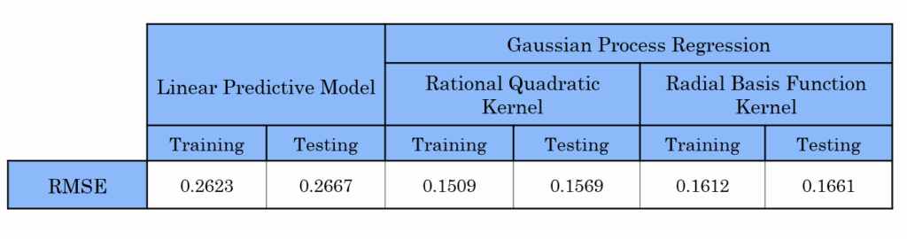
This table presents the results of our different models applied to the full training and testing datasets. As we can see, the RMSE values were best with Gaussian Process Regression, especially with the Rational Quadratic kernel. This indicates that this model provides the best fit to our actual output data.
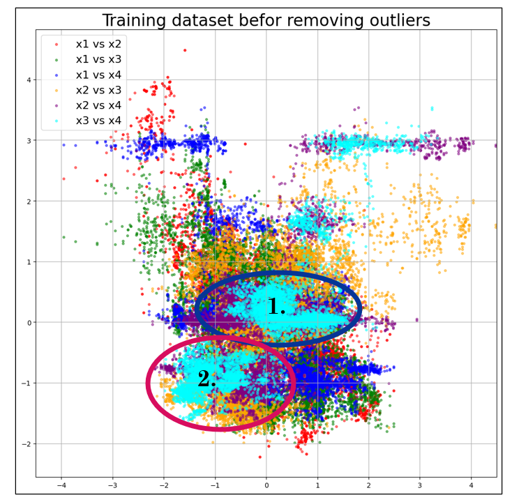
We then shifted from a general approach to an informed selection strategy, focusing on modeling a specific subset of the data.
We chose to define two clusters, as the plot reveals a noticeable concentration of data points in two distinct regions. These clusters are formed due to the behavior of variable No. 4, which represents the composition of the feed. After designing predictive models for each cluster, they can be used to predict specific subsets of measurements in the future.
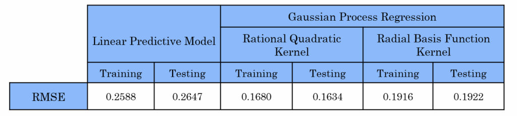
This table presents the modeling results for Cluster No. 1, which corresponds to the first region of high data density. The model shows high accuracy on both the training and testing datasets.
The next table presents the modeling results for Cluster No. 2. As shown, linear regression performs poorly in this case — the predictions significantly deviate from the actual values. This indicates that the linear model is not suitable for prediction in this cluster.
We assumed that trying to predict Cluster No. 2 using our other models might show some improvement. However, the linear model did not perform better — neither in the general approach model nor in the Cluster No. 1 model. In fact, the performance of the nonlinear models worsened in this case.
We eliminated unsuitable sensors and removed outliers. Then, we successfully designed predictive models for the alkylation process using linear regression and Gaussian (nonlinear) regression. First we applied a general approach, where we predicted the entire range of values. The best-performing model was Gaussian Process Regression with the Rational Quadratic kernel. This regression model also achieved the highest accuracy in predicting Cluster No. 1.The biggest challenge appeared with Cluster No. 2, especially when using linear regression. This led us to test different predictive models specifically for Cluster No. 2. However, similar to before, linear regression again yielded the worst results.